Understanding Quantization Effects of FIR Filter Coefficients #
In practical implementations, FIR filter coefficients are often represented with finite precision, which introduces quantization effects. In this article, we will examine the quantization effects of FIR filter coefficients using Python and MATLAB code, focusing on a low-pass filter design with specific specifications, and analyze the impact of quantization on filter performance.
Filter Design Specifications
Let’s consider a low-pass FIR filter design with the following specifications:
- Sampling frequency (Fs): 180 kHz
- Passband frequency (f1): 10 kHz
- Stopband frequency (f2): 14 kHz
- Passband ripple (R1): 0.1 dB
- Stopband attenuation (R2): 80 dB
We will estimate the filter length using the Fred Harris rule of thumb:
$$N = \frac{F_s}{\Delta_f}\frac{Atten(dB)}{22}$$
where
- \(F_s\) is the sampling rate
- \( \Delta_f \) is the transition bandwidth
- \(Atten(dB)\) is the stopband attenuation
Filter design in Python #
import numpy as np
import matplotlib.pyplot as plt
from scipy.signal import remez, freqz

# Filter specifications
Fs = 180e3  # Sampling frequency (Hz)
f1 = 10e3  # Pass band edge frequency 1 (Hz)
f2 = 14e3  # Pass band edge frequency 2 (Hz)
R1 = 0.1  # Pass band ripple (dB)
R2 = 80  # Stop band attenuation (dB)

# Estimate filter order using Harris rule of thumb
delta_f = f2-f1  # Transition bandwidth (Hz)
N = np.ceil(Fs / delta_f * R2 / 22)  # Filter order estimation using Harris rule of thumb

# Design the filter using Remez algorithm
f = [0, f1/2, f2/2, Fs/2]  # Frequency vector (Hz)
a = [1, 0]  # Desired amplitude vector
h = remez(int(N), f, a, fs=Fs)  # Filter coefficients

# Quantize filter coefficients to 8 bits
n_bits = 8
quantized_coeffs = np.round(h * (2**(n_bits - 1))) / (2**(n_bits - 1))

# Calculate quantization error
quantization_error = quantized_coeffs - h

# Plot quantization error and its spectrum
plt.figure()
plt.subplot(2, 1, 1)
plt.plot(h, label='Original Coefficients')
plt.plot(quantized_coeffs, label='Quantized Coefficients')
plt.xlabel('Coefficient Index')
plt.ylabel('Coefficient Value')
plt.legend()
plt.subplot(2, 1, 2)
w, h_quantization_error = freqz(quantization_error)
plt.plot(w, 20 * np.log10(np.abs(h_quantization_error)),label='Quantization Error Spectrum')
plt.xlabel('Frequency (Hz)')
plt.ylabel('Magnitude (dB)')
plt.legend()
plt.tight_layout()
plt.show()

# Calculate frequency response of quantized and non-quantized coefficient set
w, h_coeffs = freqz(h)
_, h_quantized_coeffs = freqz(quantized_coeffs)

# Plot frequency response
plt.figure()
plt.plot(w, 20 * np.log10(np.abs(h_coeffs)), label='Original Coefficients')
plt.plot(w, 20 * np.log10(np.abs(h_quantized_coeffs)), label='Quantized Coefficients')
plt.xlabel('Frequency (Hz)')
plt.ylabel('Magnitude (dB)')
plt.legend()
plt.title('Frequency Response')
plt.grid()
plt.show()
Filter Design in MATLAB #
% Filter specifications
Fs = 180e3; % Sampling frequency (Hz)
f1 = 10e3; % Pass band edge frequency 1 (Hz)
f2 = 14e3; % Pass band edge frequency 2 (Hz)
R1 = 0.1; % Pass band ripple (dB)
R2 = 80; % Stop band attenuation (dB)

% Estimate filter order using Harris rule of thumb
delta_f = f2-f1; % Transition bandwidth (Hz)
N = ceil(Fs / delta_f * R2 / 22); % Filter order estimation using Harris rule of thumb

% Design the filter using Remez algorithm
f = [0 f1 f2 Fs]/Fs; % Frequency vector (Hz)
a = [1 1 0 0]; % Desired amplitude vector
h = remez(N, f, a); % Filter coefficients

% Quantize filter coefficients to 8 bits
n_bits = 8;
quantized_coeffs = round(h * (2^(n_bits - 1))) / (2^(n_bits - 1));

% Calculate quantization error
quantization_error = quantized_coeffs - h;

% Plot quantization error and its spectrum
figure;
subplot(2, 1, 1);
plot(h, 'LineWidth', 1.5, 'DisplayName', 'Original Coefficients');
hold on;
plot(quantized_coeffs, 'LineWidth', 1.5, 'DisplayName', 'Quantized Coefficients');
xlabel('Coefficient Index');
ylabel('Coefficient Value');
legend('Location', 'best');
subplot(2, 1, 2);
[h_quantization_error, w] = freqz(quantization_error);
plot(w, 20*log10(abs(h_quantization_error)), 'LineWidth', 1.5, 'DisplayName', 'Quantization Error Spectrum');
xlabel('Frequency (Hz)');
ylabel('Magnitude (dB)');
legend('Location', 'best');
grid on;
title('Quantization Error Spectrum');
title('Quantization Error and Spectrum');

% Calculate frequency response of quantized and non-quantized coefficient set
[h_coeffs, w] = freqz(h);
[h_quantized_coeffs, ~] = freqz(quantized_coeffs);

% Plot frequency response
figure;
plot(w, 20*log10(abs(h_coeffs)), 'LineWidth', 1.5, 'DisplayName', 'Original Coefficients');
hold on;
plot(w, 20*log10(abs(h_quantized_coeffs)), 'LineWidth', 1.5, 'DisplayName', 'Quantized Coefficients');
xlabel('Frequency (Hz)');
ylabel('Magnitude (dB)');
legend('Location', 'best');
grid on;
title('Frequency Response');
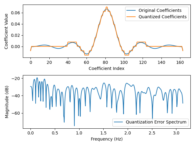
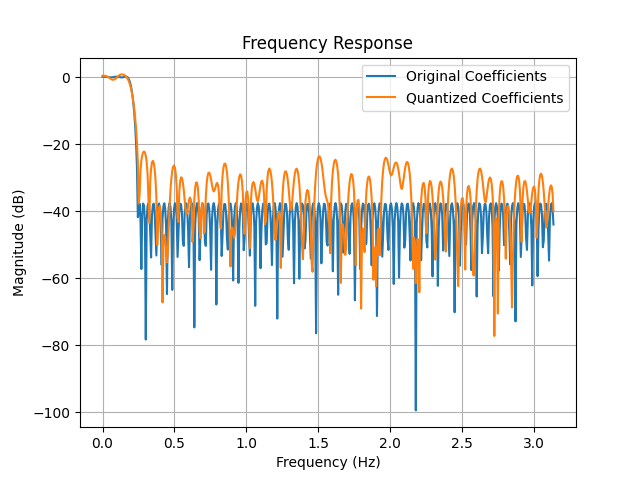
We can observe that the quantized coefficients introduce distortions in the frequency response of the filter. The out-of-band side lobe levels are increased compared to the original coefficients, leading to degraded filter performance. This is evident in the quantization error spectrum as well, where we can see additional peaks introduced due to quantization.
Quantization with Coefficient Scaling #
To mitigate the quantization effects, we can scale the filter coefficients to have unity peak gain before quantization by dividing the coefficients by the max coefficient. This approach helps to maintain the filter’s overall gain and minimize the impact of quantization on filter performance.