FIR Filter Design and Verification with Python and Cocotb #
Intro #
In the getting started tutorial we implemented a basic verilog module and simulated it with iverilog and cocotb. This tutorial will be a DSP focused look at cocotb.
What this tutorial is about #
In this tutorial we will:
- design a filter in python using numpy and scipy
- translate that design to verilog
- verify verilog implementaiton of our filter with cocotb
Design the FIR #
We need to design some filter taps to put into our verilog design, so lets do that. Lets say our filter has the following requirements:
- a passband of
+/- 0.1 * Fs - a transition of
0.1 * Fs - must be length 13
filter_design.py #
import matplotlib.pyplot as plt
import numpy as np
from scipy import signal
cutoff = .1 # Desired passband bandwidth, Hz
trans_width = .1 # Width of transition from pass to stop, Hz
numtaps = 13 # Size of the FIR filter.
fs = 1 # normalized sampling rate
# floating point coefficients
filter_coefs = signal.remez(numtaps, [0, cutoff, cutoff + trans_width, 0.5*fs],[1, 0], fs=fs)
# 8 bit integer coefficients
filter_coefs_int = np.round(filter_coefs * (2**7-1))
nfft = 2000;
print(filter_coefs_int)
x_fft = np.fft.fftshift(20*np.log10(np.abs(np.fft.fft(filter_coefs/np.sum(filter_coefs), nfft))))
xaxis = np.arange(-0.5, 0.5, 1/nfft)
x_fft_int = np.fft.fftshift(20*np.log10(np.abs(np.fft.fft(filter_coefs_int/np.sum(filter_coefs_int), nfft))))
plt.figure(3)
plt.plot(xaxis, x_fft)
plt.plot(xaxis, x_fft_int, linestyle='dashed')
plt.title('real portion of signal x')
plt.grid()
plt.xlabel('Normalized Frequency')
plt.ylabel('dB')
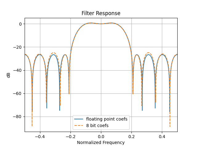
plt.title('Filter Response')
plt.xlim([-.5, .5])
plt.legend(['flating point coefs', '8 bit coefs'])
plt.show()
filter taps: [-1 -7 -4 4 18 32 38 32 18 4 -4 -7 -1]
Implement filter in verilog #
Lets implement our filter in verilog. This is not the best way (or even a good way) to design a filter in verilog, but it is a way to a implement a filter in verilog. Don’t get hung up on how incorrect or correct this is, we just want to demonstrate how to verify a complex system in cocotb.
fir.v #
module fir(clk, data_in, reset, data_out);

input clk;
input signed [7:0] data_in;
input reset;
output signed [15:0] data_out;
reg    signed [15:0] data_out_reg;

// coefficients
wire  signed [7:0]  h0,h1,h2,h3,h4,h5,h6,h7,h8,h9,h10,h11,h12;
// multiplies
wire  signed [15:0] m0,m1,m2,m3,m4,m5,m6,m7,m8,m9,m10,m11,m12;
// taps delays
wire  signed [15:0] q1,q2,q3,q4,q5,q6,q7,q8,q9,q10,q11,q12;
// adders
wire  signed [15:0] a1,a2,a3,a4,a5,a6,a7,a8,a9,a10,a11,a12;

// coefs from fir_design.py : [-1. -7. -4.  4. 18. 32. 38. 32. 18.  4. -4. -7. -1.]
// coeffs definition
assign h0  = -1;
assign h1  = -7;
assign h2  = -4;
assign h3  = 4;
assign h4  = 18;
assign h5  = 32;
assign h6  = 38;
assign h7  = 32;
assign h8  = 18;
assign h9  = 4;
assign h10 = -4;
assign h11 = -7;
assign h12 = -1;

// each multiply in the chain
assign m12 = h12 * data_in;
assign m11 = h11 * data_in;
assign m10 = h10 * data_in;
assign m9  = h9  * data_in;
assign m8  = h8  * data_in;
assign m7  = h7  * data_in;
assign m6  = h6  * data_in;
assign m5  = h5  * data_in;
assign m4  = h4  * data_in;
assign m3  = h3  * data_in;
assign m2  = h2  * data_in;
assign m1  = h1  * data_in;
assign m0  = h0  * data_in;

// each add in the chain
assign a1  = q1  + m11;
assign a2  = q2  + m10;
assign a3  = q3  + m9;
assign a4  = q4  + m8;
assign a5  = q5  + m7;
assign a6  = q6  + m6;
assign a7  = q7  + m5;
assign a8  = q8  + m4;
assign a9  = q9  + m3;
assign a10 = q10 + m2;
assign a11 = q11 + m1;
assign a12 = q12 + m0;

// delay line
dff dff1( .clk(clk), .reset(reset),.d(m12), .q(q1));
dff dff2( .clk(clk), .reset(reset),.d(a1),  .q(q2));
dff dff3( .clk(clk), .reset(reset),.d(a2),  .q(q3));
dff dff4( .clk(clk), .reset(reset),.d(a3),  .q(q4));
dff dff5( .clk(clk), .reset(reset),.d(a4),  .q(q5));
dff dff6( .clk(clk), .reset(reset),.d(a5),  .q(q6));
dff dff7( .clk(clk), .reset(reset),.d(a6),  .q(q7));
dff dff8( .clk(clk), .reset(reset),.d(a7),  .q(q8));
dff dff9( .clk(clk), .reset(reset),.d(a8),  .q(q9));
dff dff10(.clk(clk), .reset(reset),.d(a9),  .q(q10));
dff dff11(.clk(clk), .reset(reset),.d(a10), .q(q11));
dff dff12(.clk(clk), .reset(reset),.d(a11), .q(q12));

// filter output data_out[n] = conv(x[n], h[n])
always @(posedge clk)
begin
  if(reset)
    data_out_reg <= 0;
  else
    data_out_reg <= a12;
end
assign data_out = data_out_reg;

// Dump waves
initial begin
  $dumpfile("dump.vcd");
  $dumpvars(1, fir);
end
endmodule
The above verilog uses another module, dff, so you will also need to include this in your design. This is a good example for showing how to include multiple verilog files in your cocotb makefile.
dff.v #
module dff(clk, reset, d, q);
input clk;
input reset;
input  [15:0] d;
output [15:0] q;
reg    [15:0] q_r;

always @(posedge clk or posedge reset)
begin
    if(reset)
        q_r <= 16'b0;
    else
        q_r <= d;
end

assign q = q_r;
endmodule
cocotb testbench #
testbench.py #
# Simple tests for an fir_filter module
import cocotb
import random
from cocotb.clock import Clock
from cocotb.triggers import Timer
from cocotb.triggers import RisingEdge
from scipy.signal import lfilter
import numpy as np
import matplotlib.pyplot as plt
# as a non-generator
def wave(amp, f, fs, clks):
clks = np.arange(0, clks)
sample = np.rint(amp*np.sin(2.0*np.pi*f/fs*clks))
return sample
def predictor(signal,coefs):
output = lfilter(coefs,1.0,signal)
return output
@cocotb.test()
async def filter_test(dut):
#initialize
dut.data_in.value = 0
fs = 1
amp0 = 80
num_clks = 512
nfft = num_clks;
f0 = 50*(1.0/nfft)
coefs = np.array([-1., -7., -4., 4., 18., 32., 38., 32., 18., 4., -4., -7., -1.])
cnt = 0
# input data
input_signal = wave(amp0, f0, fs,num_clks) + wave(amp0/2, 200.5*(1.0/nfft), fs, num_clks)
# bit accurate predictor values
data_out_pred = predictor(input_signal, coefs)
# start simulator clock
cocotb.start_soon(Clock(dut.clk, 1, units="ms").start())
# Reset DUT
dut.reset.value = 1
await RisingEdge(dut.clk)
dut.reset.value = 0
output_signal = np.zeros(num_clks)
# run through each clock
for samp in range(num_clks):
await RisingEdge(dut.clk)
# get the output at rising edge
dut_data_out = dut.data_out.value.signed_integer
# feed a new input in
dut.data_in.value = int(input_signal[samp])
output_signal[samp] = dut_data_out
# wait until reset is over, then start the assertion checking
if(cnt>=2):
assert dut_data_out == data_out_pred[cnt-2], "filter result is incorrect: %d != %d" % (dut_data_out, data_out_pred[cnt-2])
cnt = cnt + 1
in_fft = np.fft.fftshift(20*np.log10(np.abs(np.fft.fft(input_signal, nfft))))
out_fft = np.fft.fftshift(20*np.log10(np.abs(np.fft.fft(output_signal[2:], nfft))))
pred_fft = np.fft.fftshift(20*np.log10(np.abs(np.fft.fft(data_out_pred[:-2], nfft))))
filt_fft = np.fft.fftshift(20*np.log10(np.abs(np.fft.fft(coefs/sum(coefs), nfft))))
# normalize FFTs lazy style
in_fft = in_fft - np.max(in_fft)
out_fft = out_fft - np.max(out_fft)
pred_fft = pred_fft - np.max(pred_fft)
xaxis = np.arange(-0.5, 0.5, 1/nfft)
plt.figure(1)
plt.subplot(1,2,1)
plt.plot(output_signal[2:], marker='x')
plt.plot(data_out_pred[:-2], marker='o')
plt.legend(['DUT', 'Theory'])
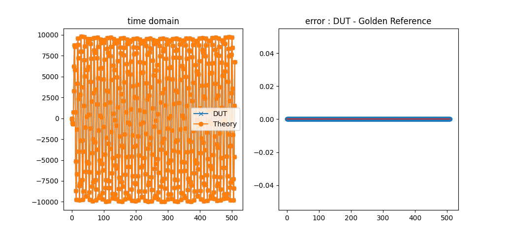
plt.title('time domain')
plt.subplot(1,2,2)
plt.stem(output_signal[2:]-data_out_pred[:-2])
plt.title('error : DUT - Golden Reference')
plt.figure(2)
plt.subplot(2,1,1)
plt.plot( xaxis, in_fft)
plt.plot(xaxis, filt_fft)
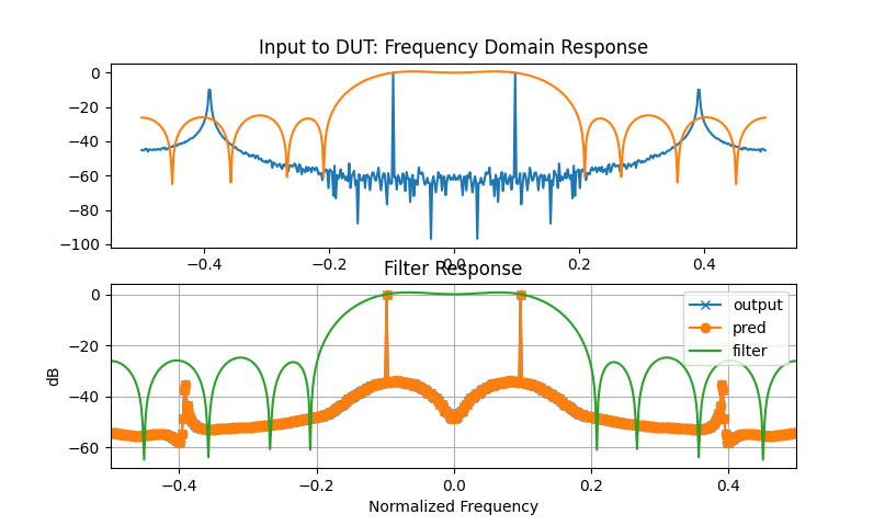
plt.title('Input to DUT: Frequency Domain Response')
plt.subplot(2,1,2)
plt.plot(xaxis, out_fft, marker='x')
plt.plot(xaxis, pred_fft, marker='o')
plt.title('Output of DUT: Frequency Domain Response')
plt.plot(xaxis, filt_fft)
plt.grid()
plt.xlabel('Normalized Frequency')
plt.ylabel('dB')
plt.title('Filter Response')
plt.xlim([-.5, .5])
plt.legend(['output', 'pred', 'filter'])
plt.show()
makefile #
# defaults
SIM ?= icarus
TOPLEVEL_LANG ?= verilog

VERILOG_SOURCES = $(PWD)/*.v

# use VHDL_SOURCES for VHDL files

# TOPLEVEL is the name of the toplevel module in your Verilog or VHDL file
TOPLEVEL = fir

# MODULE is the basename of the Python test file
MODULE = testbench

COCOTB_HDL_TIMEUNIT = 1ns
COCOTB_HDL_TIMEPRECISION = 1ps
# include cocotb's make rules to take care of the simulator setup
include $(shell cocotb-config --makefiles)/Makefile.sim
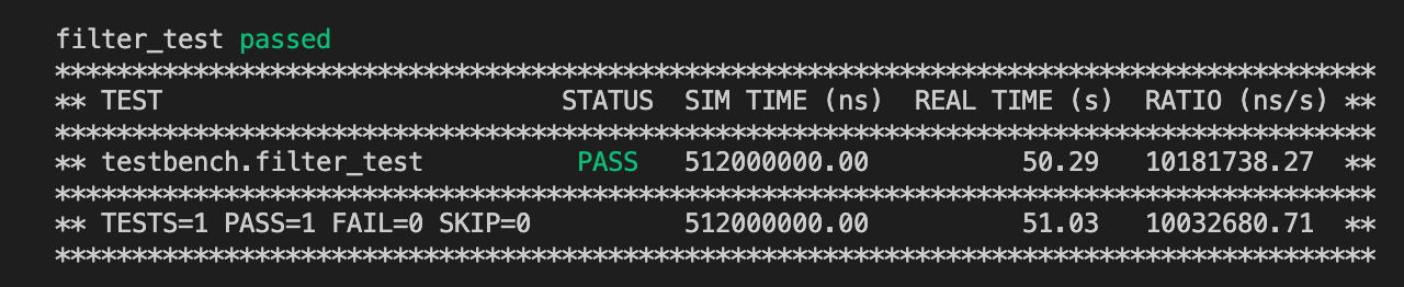
results #
Frequency Domain Plots:
Time Domain Plots:
Regression/Assertion Checks: