Building an OFDM Modem that Operates in the Audio Spectrum Part 1 #
This project is about building the physical (PHY) layer of an OFDM modem that works over audio. OFDM is used in WiFI, 5G, digital TV, and a host of other radio communincation.
Maybe we will build the upper layers of the stack eventually
Part 1 Video #
Live coding of part 1 for bedtime:
Code #
Part 1 Goals/Requirements #
✅ Write the following blocks in the processing chain:
- IFFT
- cyclic prefix application
- interpolation
- frequency shift
✅ Write functionality to create OFDM symbols with:
- configurable FFT size
- cyclic prefix length
✅ Write functionality to transmit OFDM symbols in the audio spectrum with configurable:
- baseband sampling rate
- transmit sampling rate
- transmit center frequency
Intro #
OFDM is a method for digital communications using a frequency multiplexing scheme that uses multiple sub-carriers to transmit several symbols of data in parallel. Each sub-carrier can use a common modulation scheme such as quadrature amplitude modulation or phase shift keying. The advantages of OFDM lies in its straight-forward channel equalization scheme, easy elimination of inter-symbol interference, and efficient implementation via the FFT [1].
The OFDM Transmitter #
After passing through the channel it is the OFDM receivers job to correct for unideal characteristics in the received signal. Some important aspects of proper reception include: synchronization (which includes packet detection, timing recovery, and carrier frequency offset correction) and channel equalization. The general flow of data is summarized in the figure below.
scroll---->
+-----------------+         +-----------------+          +-----------------+          +-----------------+          +-----------------+          +-----------------+          +-----------------+
|                 |         |                 |          |                 |          |                 |          |                 |          |                 |          |                 |
|                 |         |    MAP TO       |          |                 |          |                 |          |                 |          |                 |          |                 |
|   DATA STREAM   |--------->    MODULATION   |--------->|      IFFT       |--------->|  CYCLIC PREFIX  |--------->|   INTERPOLATE   |--------->|    FREQUENCY    |---------->   DIGITAL TO    |
|                 |         |    SCHEME       |          |                 |          |                 |          |                 |          |    SHIFT        |          |   ANALOG        |
|                 |         |                 |          |                 |          |                 |          |                 |          |                 |          |                 |
+-----------------+         +-----------------+          +-----------------+          +-----------------+          +-----------------+          +-----------------+          +-----------------+
Sub-Carriers and Orthogonality #
After mapping the data to a complex constellation, the data is then fed in parallel to 1 of the N subcarriers in IFFT. Due to the properties of the IFFT, the IFFT of the mapped data will be a summation of orthogonal sinusoids in the time domain [1]:
$$x_{tx}(n) = \sum_{k=0}^{N-1} X(K) e^{\frac{j2 \pi n k}{N}}$$
In Equation above \(X(K)\) is the constellation point mapped to the sub-carrier (or frequency bin) \(K\). The variable \(N\) is the Fast Fourier Transform (FFT) size, and \(x_{tx}(n)\) are the time domain samples after the IFFT. Orthogonality of frequency division is achieved through selection of a sub-carrier distance \( \Delta f\) which is the reciprocal of sampling time, \(Ts\) times the number of sub-carriers in the design, \(N\) [1]:
$$\Delta f = \frac{1}{NT_s}$$
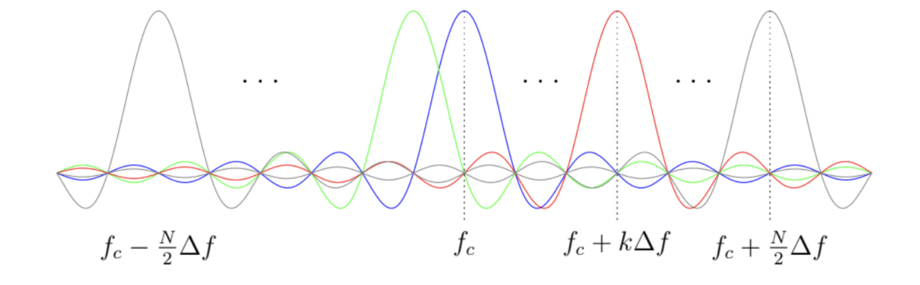
In a 4KHz bandwidth system with 64 sub-carriers, each sub-carrier is then spaced 62.5 Hz apart. A visual representation of the orthogonal sub-carriers is further explained by the figure below, which shows the \(N\) orthogonal sub-carriers in the frequency domain, each with \(k \Delta f\) spacing where \(k = \frac{-N}{2}, -\frac{N+1}{2},…,\frac{N}{2}\)
In first part 1 of the youutbe series we performed some simple test of the processing chain by filling up nearly half our IFFT bins (the positive portion), taking the IFFT of the signal and then taking the FFT again to sanity check the functionality. The baseband sampling rate is 4KHz, and the FFT below spans +/- 2KHz, as expected.

Cyclic Prefix #
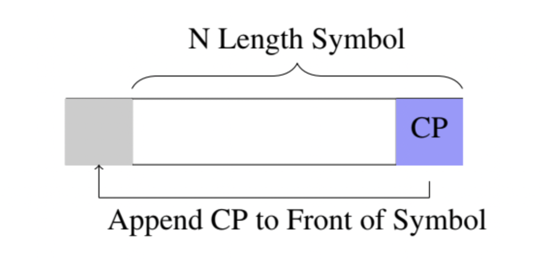
After transforming the digitally modulated constellation to a time domain signal, the next step is to reduce the time-dispersive effects of the channel that would cause inter-symbol interference (ISI). This is accomplished by prefixing a guard interval called the cyclic prefix (CP) to the samples as seen in the first figure below. The guard interval duration is denoted \( T_{guard}\) where the total length of the symbol is \(T_{sym}\). The \( \frac{T_{guard}}{T_{sym}}\) ratio is typically \( \frac{1}{4}\). The total symbol duration then becomes \(T_{total} = T_{sym} + T_{guard}\). The guard interval serves to reduce the unwanted channel dynamics [2] wherein energy between OFDM symbols leaks causing ISI and loss of orthogonality between sub-carriers.
A simple way to picture this is that even if receiving FFT is misaligned, the cyclic prefix makes sure that all samples come from the same symbol.
scroll ---->
      +---------+-----------------------+---------+-----------------------+---------+-----------------------+
      |CYCLIC   |  OFDM SYMBOL 0        |CYCLIC   |  OFDM SYMBOL 1        |CYCLIC   |  OFDM SYMBOL 2        |
      |PREFIX 0 |                       |PREFIX 1 |                       |PREFIX 2 |                       |
      +---------+-----------------------+---------+-----------------------+---------+-----------------------+
                +-----------------------+         +-----------------------+         +-----------------------+
                |     FFT WINDOW (RX)   |         |     FFT WINDOW (RX)   |         |     FFT WINDOW (RX)   |
                +-----------------------+         +-----------------------+         +-----------------------+
              +-----------------------+         +-----------------------+         +-----------------------+
              |     FFT WINDOW (RX)   |         |     FFT WINDOW (RX)   |         |     FFT WINDOW (RX)   |
              +-----------------------+         +-----------------------+         +-----------------------+
         +-----------------------+         +-----------------------+         +-----------------------+
         |     FFT WINDOW (RX)   |         |     FFT WINDOW (RX)   |         |     FFT WINDOW (RX)   |
         +-----------------------+         +-----------------------+         +-----------------------+
Interpolation/Upsampling #
What a lot of books don’t talk about in the context of OFDM is how to get from you baseband signal to actually transmitting it. They make assumptions that a magical machine teleports your baseband signal to the correct center frequency, but a couple things need to happen, the first of which is interpolating your baseband rate to your transmitting frequency rate.
In tinyofdm, we typically use about 4KHz for baseband and will transmit to our soundcard at the soundcards sampling rate. Typical audio sampling rates are 44.1KHz, 48Khz, 96Khz, and 192KHz. So we need to resample the baseband signal from 4KHz to one of these audio sampling rates. To do this you could design polyphase filters to do the job, but tinyofdm takes a minimal approach and uses scipys resample function.
Resample x to num samples using Fourier method along the given axis.The resampled signal starts at the same value as x but is sampled with a spacing of len(x) / num * (spacing of x). Because a Fourier method is used, the signal is assumed to be periodic.
This is a quick and easy way to get the job done, perhaps in future iterations we will redo it with polyphase filters.
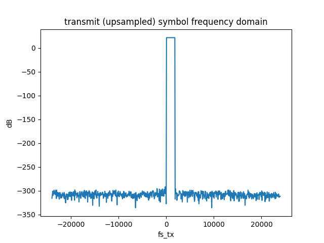
In the video, a test was run to make sure the upsampling worked as expected. We expect to see the baseband OFDM spectrum (+/- 2KHz, of which only half the spectrum was used ~2KHz). The output of the upsampling function should have our original signal, but at the new sampling rate of 48KHz - the soundcards sampling rate:
Frequency Shift to Carrier Frequency #
The last step in the process is to shift our interpolated/upsampled signal from baseband to the carrier frequency.
The baseband signal coming out of the IFFT is a complex signal. Your soundcard, like most transmitters, cannot consume complex data so we need to convert the complex data stream into one signal (you can think of the complex signal as two signals). We basically want to add the real and imaginary portions of our complex signal and then transmit them out of the speaker.
This addition is called quadrature mixing. In tinyofdm the following operation is performed:
$$ real(x_{tx}(n) * e^{j 2 \pi f_c n})$$
if we break that down we have:
$$[ x_{tx}^{real}(n) + j x_{tx}^{imag}(n) ][lo^{real}(n) + j lo^{imag}(n)]$$
where \(lo\) is our local oscillator \(e^{j 2 \pi f_c n}\). If we follow the math through:
$$ x_{tx}^{real} lo^{real} - x_{tx}^{imag}\cdot lo^{imag}$$
That is to say the below python code would have accomplished the same thing:
dti = np.real(data) * np.cos(2 * np.pi * self.fc/self.fs_tx * samples)
dtq = np.imag(data) *-np.sin(2 * np.pi * self.fc/self.fs_tx * samples)
xtx = dti + dtq
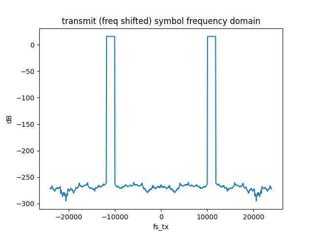
This functionality was also sanity checked in part 1 of the video. Since we go from complex to real we expect images in both Nyquist Zones. The baseband signal was frequency shifted to 10KHz, as can be seen below:
A Cursory Overview of Wireless Propagation and Multipath Effects #
Once the signal has left the transmitter (the speaker in tinyofdm’s case) it will encounter numerous effects due to the channel. These include linear and nonlinear effects which must be accounted for in the receiver if the signal is to be recovered. This section will not be a rigorous study into the channel distortion, but will highlight distortion phenomena which are relevant.
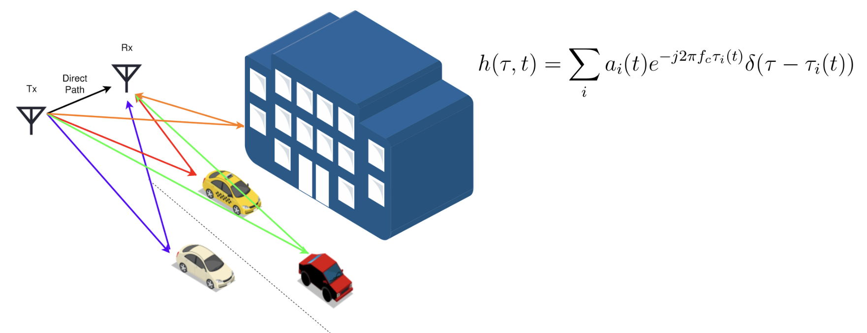
The most relevant distortion to audio, perhaps, is multipath interference which occurs when the direct signal path between the transmitter and receiver encounters distortion from signals arriving at the receiver with different amplitude and delays. In the audible spectrum this would mean a very echo-y room where you receive slightly delayed versions of your signal from different reflections. This introduces gain and phase distortions in the received signal[2].
Multipath propagation can cause non-ideal magnitude and phase characteristics which causes dispersion in the time domain transmitted signal. Dispersion occurs when the transmitted signal spreads out in time as it propagates through the channel due to unideal characteristics. Frequency division multiplexing schemes are typically robust against dispersive effects of a channel due to clever ISI reduction techniques employed by the addition of the cyclic prefix. Addition of the CP allows pulse spreading to occur without detrimental interference to neighboring channels.Nevertheless, while robust, these effects still take place and can be seen in an OFDM system.
One other important effect caused by channel distortion is channel fading. Two or more signals (due to multipath effects) can cause constructive or destructive interference, effectively changing the gain of the received signal [2]. Channel fading can be strongly frequency dependent, but equalization in OFDM can remove these detrimental issues.
References #
[1] A. Goldsmith, Wireless Communications. Cambridge, U.K.: Cambridge University Press, 2004.
[2] B. P. Lathi, Modern Digital and Analog Communication Systems 3e Osece, 3rd ed.Oxford University Press, 1998.